Timing Is (Almost) Everything
Timing Is (Almost) Everything
With almost everything in life there is an element of seasonality to be considered before embarking on a particular activity, journey, or mission. For instance, when attempting to ascend a previously unconquered mountain you most likely want to first observe weather patterns throughout several seasons and then pick the best route at the best time – which combined will increase your odds of reaching that coveted peak. When planning a trip to Paris you will most likely consider spring or autumn instead of the dead of winter. Skiing in the Austrian Alps is best enjoyed in late fall or early spring and you won’t be finding many operating skilifts in mid June. So we can all agree that the concept of seasonality is deeply ingrained in our human nature and culture as it roots back throughout the millennia all the way to the very dawn of life on this planet.
As the financial markets are largely driven by human nature and human psychology it thus not surprising to observe a cyclical dimension which many scholars have devoted much time and effort quantifying. Ralph N. Elliott for instance is famous for his study of the wave principle in stock markets that is known today as the Elliot Wave Principle. In his comprehensive work he identified fractal bull and bust cycles which he recognized as patterns that appear to repeat themselves on various time intervals, from just a few minutes all the way to years, decades, and even centuries. Chris Carolan, a friend of the blog, wrote a fascinating book called the Spiral Calendar, which defines time intervals from a derived Fibonacci series based on moon cycles (29.53 days). The basic Spiral Calendar thesis is that emotional market turns are linked to past emotional market turns by Spiral Calendar time units in quantities greater than random. Although this may all sound highly exotic to the unexposed reader I would strongly recommend Chris’ work, which since has evolved into defining Solunar models for various markets (i.e. Dow, Gold, etc.). As a matter of fact much of what Volar and I present here today has been confirmed by Carolan’s work, despite the fact that Volar’s charts are purely statistical in nature. It’s always fascinating and a bit rewarding to have your own work supported by a completely different theory.

To boot here is a basic concept chart Volar produced a few weeks back – I really like how he used color codes to represent four main seasons throughout the trading year. As you can see we just entered the ‘vacation’ season and historically it averages to the downside. When compared to the 200-day SMA the rate of ascend during the vacation season is rather mild when compared with the Holidays or Easter seasons.

It thus no surprise to see this basic seasonality reflected in the chart above. Apparently being long between March – April, during July, and then again from October all the way through January appears to have clear statistical support. And yes, to my very own surprise October is often a pretty good month – once you exclude the 1987 and 2008 crashes.
But wait – we’re only getting warmed – go grab a cup of tea or java, there are plenty of charts to go:
[amprotect=nonmember]
Charts and commentary below for anyone donning a secret decoder ring. If you are interested in becoming a Gold member then don’t waste time and sign up here. And if you are a Zero subscriber it includes access to all Gold posts, so you actually get double the bang for your buck.
[/amprotect]
[amprotect=1,9,5,2]

S&P easonality measured since 1950 clearly shows the good (DEC, APR, NOV, MAR), the bad (MAY, AUG), and the ugly (SEP, FEB, JUN). But Mole – why are you calling SEP, FEB, and JUN, the ugly? After all, a down month can be a very good month if you happen to be shorting the market! Well, although there appear to be clearly positive cycles you will soon see that there are no clear negative cycles. Volar was able to identify several months with a slightly negative slant but I was not able to identify a clear edge.

This shows the average percentage of return had you been long the S&P. It doesn’t take a sophisticated pattern analysis algo to identify which weeks of the year have been statistically positive for the past sixty years. This greatly reflects my own observations over the years (and that of my peers) and as such the old trader adage ‘Go away in May’ seems to hold a lot of truth. Those old ticker reading pit traders apparently knew a thing or two about seasonality.
Before you all cancel your subscription for the next four months I must however point out that ‘no edge’ does not necessarily mean ‘no profits’. And the chart above supports my intention to start covering delta neutral option strategies in the coming months. Just because price isn’t moving in a clear direction it doesn’t mean we can’t be selling theta or vega. After all there are many ZH reading doom sayers willing to buy vega after a strong push to the upside 😉

I actually saw this chart after I had highlighted the previous one myself – apparently Volar seems to be on the same page when it comes to picking ‘easy money periods’. Sharpe Ratio reflects the ratio of return in relation to standard deviation and again weeks 10-19 and 44 to 1 stand out. The lessons for the bears: Don’t be short during these periods! The lesson for the bulls: Don’t waste theta with long term calls starting in mid May.

This chart again plots positive growth expectations in percentage terms. To be clear – we are not looking at the odds of growth but the average percentage of grown. Again, it seems that late Apri, May and December are non brainers for the longs. I don’t see a clear cluster of negative growth for the bears however – where there are successive down bars the intensity does not justify taking the risk IMNSHO.
Lesson learned: Life is tough for a bear.

Since it’s June let’s analyze performance cycles across the last 60 years. Volar seems to think that there is a six year cycle and maybe he’s right. I would however prefer to see the more consistent months being plotted like this. How about it Volar – can we make this a follow up post for next Sunday? 😉

Trading range – a.k.a. ATR: Although December appears to be a no brainer for the longs there appears to be limited trading range due to the holidays. October produced two crashes in the past quarter century so I’m not surprised it pops out a little. But the real fun happens in January and that actually in the first week or two. Usually there is a ramp followed by a drop in the second or third week, plenty of opportunities to play the swings and we should mark our calendars. As you can see February just outright sucks – depending on your perspective – if you love delta neutral strategies then February is your ticket. Volar – I would love to see a VIX correlation analysis relative to February and December – could be valuable in the context of volatility plays.

Here we are looking at the average return on long trades on a monthly basis. March and April is where the money is – so is October through January. And yes, we are now in one of the lousiest months of the year for directional plays and thus we better start covering some smart option plays that leverage sideways tape. Any option addict takers?

Directional bias means deviation from the current trend. Actually I’d be really curious as to how Volar calculated this one as the math can be quite complex. The main trend needs to be defined and quantified, after which you calculate the skew. October again stands out with two party surprises in the past quarter century. Lesson learned – markets love to crash in fall. However bear in mind that October can also be a good month. So, second lesson learned: October can be good to the bears – but when it’s not it gets really ugly. Let’s call October the year’s PMS month (my apologies in advance to any female readers).

If you take each month on its own this chart shows how many of the last sixty were positive on a percentage basis. Again, December is the no-brainer for the longs, no matter how we look at it, closely followed by April. September apparently is on the bottom of the pack, but let’s not forget that this is NOT a complete bar, anything below 42% is cut off. Meaning all months in the last sixty years were positive at least 44% of the time. If you do the math this comes out to 26 months out of 60.

Analog years are those that resemble the current year in direction and form – Volar picked five candidates that appear to have followed a similar path as 2011. Based on those analogs we are looking at a sideways summer and a bullish fall. Of course our mileage may vary – this does not mean we can’t suddenly change directions, in which case Volar would have to map 2011 to other analog years. Hope this makes sense.

Feel free to use this chart as a pattern for your next wall paper. As you can see we are looking at the same analogs (plus 1997) but the respective lines plot a 25-day SMA of CBOE call/put activity. I assume Volar uses call/put instead of put/call plots to map it to directional/price moves in the S&P (please feel free to correct if I got this one wrong).

The AAII is a popular sentiment measure published by the American Association of Individual Investors. Volar selected years with a bullish bias and lined them all up with each other. The problem with this chart is that the swings make it difficult to make a proper correlation so I asked him to index it differently.

And that was the result – isn’t that a lot better? As you can see creating order on a chart sometimes requires shifting plots against each other and unfortunately I don’t know of a single charting package that supports that. I guess I could write my own – my TOS left chart script could be extended to accommodate some type of vertical indexing.
I hope you all enjoyed this post and perhaps store is as a bookmark for future reference. In addition to system discipline, capital commitment guidelines, market exposure weightings, and stop loss provisions it seems that seasonality potentially can give us that extra edge for picking the most effective trading strategies at the proper right time. I strongly encourage discussion and proposals as to how we can leverage this data in the coming weeks and months. After all I can’t do it all on my own 😉
Many thanks to Volar for producing this set of charts – quite frankly this quality of analysis is usually not available to retail traders and institutions pay thousands of Dollars for this type of data. We are all grateful for your contributions, Volar – keep up the good work.
Cheers,
Mole
[/amprotect]