Figuring Out How Wrong You Are

This post was inspired by a Quantopian lecture I greatly enjoyed this weekend and which once again confirmed to me that even the most basic tools and measures taught in the vast majority of educational trading material merely give us a momentary snapshot of the whole underlying picture. To take any statistical or technical parameter at bare face value is akin to judging an entire movie by a single frame or a composition by a single note. So let’s put those 3D glasses on and learn how to dig a little deeper, shall we?

Alright we pretend that we have a very simple trading system which has but one single rule: Be long AMZN without a stop or a target. Simple enough and it serves us well for demonstration purposes as our P&L now effectively becomes the price series of Amazon. We are going to buy Amazon on 1/1/2012 and hold it through 1/1/2015 – four years of continuous price action.

Sharpe Ratio

Now one statistic often used to describe the performance of an asset or a trading system is the Sharpe ratio. Actually there are two – a more simpler one that compares the mean of your returns to the standard deviation of your returns – and one that uses an additional ‘risk free’ baseline measure such as for example the return of a treasury bill. All we need to do is to calculate the difference between our system returns and the returns of the ‘risk free’ treasury bills – let’s call that our risk_only series. Then we divide the mean of the risk_only series by the standard deviation of the risk_only series, and we’re done.

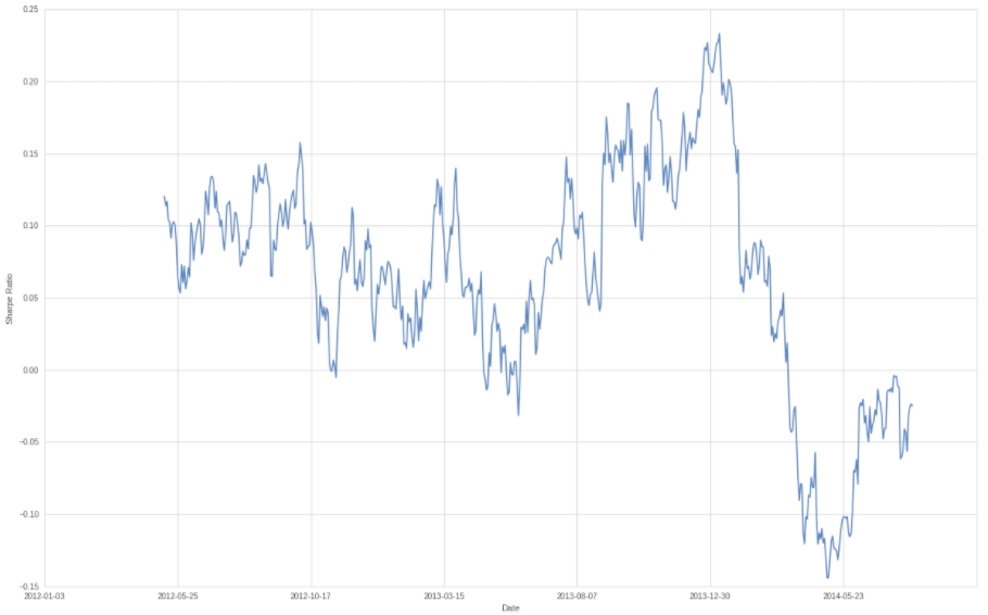
Of course calculating a sharpe ratio for the entire four years or even an entire year doesn’t really give us an accurate view of how well our system performs on an ongoing basis. For our purposes we are going to use a running window of 90 days, which is shown in the chart above. Well, that Sharpe ratio is looking rather volatile isn’t it? Which teaches us that reporting just a single value isn’t very helpful for predicting future system returns.

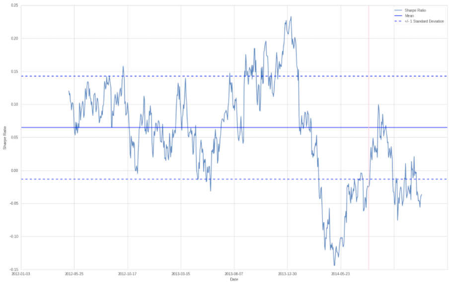
To give us a better idea we’re going to calculate the mean and the standard deviation of our Sharpe Ratio. We are using a 1.0 range up and down and plot that on top as to get a better understanding how volatile returns can be. And what we are learning is that it varies hugely and thus calculating a Sharpe ratio at any moment in time only gives us a fraction of the information. I could be building a system and test it back a year or two and when calculating the annual Sharpe I may be getting a very positive value and then six months later get a negative one. Sure getting a very positive averaged annualized Sharpe throughout an extended testing period is a good thing. But it does not tell us anything about the volatility that got us to that point. SQN implicitly fixes that problem to some extent (as it considers standard deviation and opportunity) but knowing what I know now I would still plot it a a rolling window.

 Moving Averages

Many of us are using moving averages on a daily basis but rarely consider what it really represents. Yes, just as its name suggests it is a price average measured within a forward sliding window. Let’s plot a 90 day average and then consider what it’s telling us:

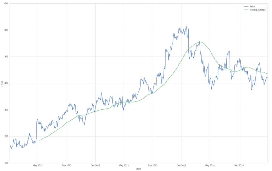
Yes yes, I know what you’re thinking. Mean reversion and all but what if you’re shifting the mean by adjusting the window? What is the perfect moving average? Well, frankly there is none because like all derivatives of price it suffers from auto correlation and residuals, which are basically your errors.

The perfect moving average has a width of 1 as it tracks price perfectly – from there we are starting to average and thus we are amplifying the distribution of our errors (i.e. the distance between price and our moving average). Let that sink in for a moment and then take a look at the chart above which plots a rolling window measuring the standard deviation of our price series. Clearly we are seeing quiet periods and rather volatile ones. So how volatile is our price series or the returns of our trading system? Very tough to say – the less volatile the better, right? But auto correlated historical series which follow a random walk it is very difficult for us to establish one concise measure that is universally applicable.

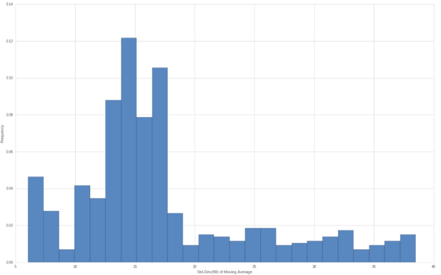
Remember that the larger our moving average window the larger the average standard deviation but also the more skewed the distribution of errors. Shown above is the rolling 90-day standard deviation of our system (in this case the price returns of NFLX) as a histogram. Note that the peak values are below 40 here but that the majority of the values are distributed between 10 and 20.

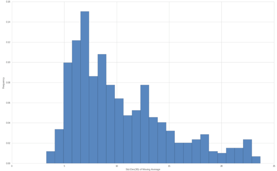
And here for comparison is a histogram of the rolling 30-day standard deviation. As expected the peak values are less pronounced now fizzling out blow 25 while the majority of the values are clustered between 5 and 10. So our std dev profile narrowed and flattened a little but our distribution appears more platykurtic.

Of course both histograms are based on the very same return series (in this case a simple price series) and thus our perspective once again is based on whatever sliding window we are choosing. In other words both histograms show us the very same return profile but from a different perspective. No matter which perspective you choose however, anything is better than just one single value.

Conclusion

Whenever we compute a parameter for any data set we need to also compute its volatility. Otherwise we do not know how far future measures deviate from the summary value we have just computed. The general strategy is to divide the data into subsets or sliding windows and then calculate a series of parameters instead of just settling on just one.