Quantutorial – Standard Deviation

Standard deviation. You see it mentioned all the time but if that inquisitive little niece of yours would ask you what it is, could you actually explain it? No, I’m not talking about googling the formula on your mobile and then telling her to scram and kick a ball or something. What I mean is explaining standard deviation (SD) in a way that actually makes sense and may lead to her to taking an interest in STEM sciences later in life. Yeah, I didn’t think so. And you call yourself a trader? Step aside and let uncle Mole handle this.

Alright Lucy (that’s her name), imagine you take your ball into the yard outside and start kicking it. Every time you kicked it you measure the distance. Warning: Since Lucy is a spoiled little American brat we’ll be talking about yards – which will cause European metric based children to experience instant cerebral hemorrhage. So you kicked it the first time and it went 10 yards. You write that number down and then kick it again. Unfortunately you tripped a little and so the ball only went 3 yards. It counts anyway so write it down. Next time you take a running start and the ball flies 20 yards. Excellent, that definitely gets recorded for posterity. Meanwhile your annoying little brother shows up and kicks the ball away from you. He’s half your size so it only went 6 yards but he kicks it again and scores 8. You run after the little bugger and kick it back about 12 yards. Who instantly starts bawling and just out of spite kicks that ball as far as he possibly can – 9 yards – through the kitchen window. Game over and of course you blame your brother for everything.

So let’s do the numbers – we have measured 7 kicks in yards:

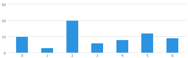
10, 3, 20, 6, 8, 12, 9

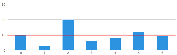
First we need to figure out the average or mean of the distances, which we get by adding all those numbers together and dividing it by 7. So that would be 68 divided by 7 which yields us 9.71. Let’s draw a line on our chart:

Alright at this point it’s becoming clear that Lucy must have been feeding her ADD meds to her dog as she ran out to play about five minutes ago. Mental note to drop her from this year’s Christmas shopping list. So let’s explain the rest to that good-for-nothing brother of yours:

All we do from here is to deduct the mean (i.e. 9.71) from all the numbers:

0.29, -6.71, 10.29, -3.71, -1.71, 2.29, -0.71

Oh-ooooh – negative numbers. I don’t remember anyone kicking the ball backwards! What to do? Simple we square those numbers which gets us a positive series:

0.08, 45.08, 105.80, 13.80, 2.94, 5.22, 0.51

Now that’s weird. Seems like the negative numbers turned into very large exponents. Those are actually the relative ‘variances’ based on the mean and if we take the mean of all those numbers we get to… drum rolls… 24.78. That number represents the average variance from the mean.

So how about standard deviation? I got you covered. All you need to do is to square that number and you get to 4.987, which is the standard deviation. Finally!

Of course one really annoying thing about that imbecile of a brother is that he never trusted you. So he whips out his mobile phone and goes to an online SD calculator. ‘Ha-haaa!’ he shouts ‘you were wrong!! See here, the real standard deviation is 5.376. I knew you always sucked in math’.

Ooops that’s embarrassing, what happened? Well, tell your brother that he calculated the ‘sample SD’ while you gave him the ‘population SD’. What’s the difference? If you take only a sample from a larger population of numbers then you need to actually deduct 1 from the number samples when calculating your variance. Instead of dividing the sum of the squared values by 7 we divide them by 6.

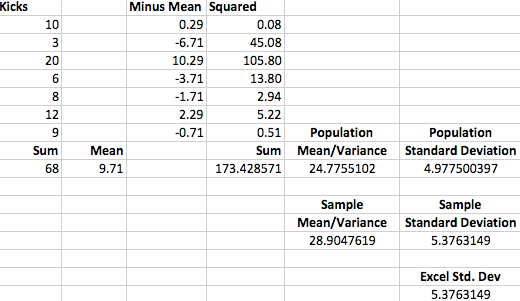
Here’s a spreadsheet I put together so you don’t get confused. On the bottom left you see our ‘control number’ which Excel’s built-in SD function. So we are spot on!

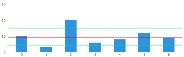
All that’s left to do for us now is to actually draw the SD value(s) to our chart, in this case a very simple bar graph. Just like with a Bollinger you take the mean and then add the SD of 5.37. For the negative SD you simply deduct the same SD. That gives us two lines shown above in green, one at 4.338 and another at 15.09 (for sample SD which is what everyone uses by default). If you count the numbers of bars (i.e. kicks) that fall within that standard deviation range you arrive at 5 out of 7 (the 2nd and 3rd are outside). That sounds about right as that is 71% within a very small sample of 7. Strangely when writing that little story for Lucy I just pulled those numbers out of my butt and it’s interesting that the numbers worked out so well. So there appears to be a natural and almost instinctive order to distribution patterns.

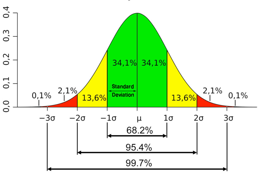
Now if Lucy raided her mom’s cookie jar and due to an epic sugar rush kept kicking that ball for hours on end whilst collecting the distances odds suggest that the final tally would settle around 68% – a little over 2/3 of the sample size. Another way of phrasing it is that 68% of all the kicks would most likely fall within a standard deviation range of 4.338′ to 15.09′. And that is called ‘normal’ distribution or ‘Gaussian’ data.

But wait there is more. We can actually keep adding SD intervals simply by adding the same distance (i.e. 5.37) once again and then again. Which is visualized in the graph shown above – I’m sure you’ve come across it in the past. In this specific case the kicking range spanning 2 standard deviations would be between 0.87′ to 18.558′ and encompass over 95% of all the samples. Each standard deviation interval is also often referred to as ‘confidence intervals’ and that is what the nerds mean by ‘sigma’.

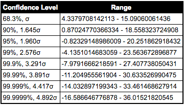
Here’s a handy table that shows you each confidence interval, assuming normal distribution (a topic we have covered in the past but will revisit in the near future). If you click on the table it’ll get you to the page where you can play with the numbers or add your own.

Six Sigma Event?

Remember last time when you read some article over on ZeroEdge suggesting the possibility of a ‘six sigma’ event? Well, if you count the rows in that table above then you realize that this puts us in the top 0.001% of all trading days, which is 1/1000th of one percent, or one out of 100,000. Wait a minute. 100,000 / 365 comes out to 273 years? Almost three centuries? But we had several major market crashes in the past 100 years alone, not even counting recent flash crashes:

1. Florida Real Estate Craze in 1926
2. The Great Depression starting in 1929
3. The Big Crash of 1987
4. The Asian Crisis starting in 1989
5. The Dotcom Crash in 2000
6. The Housing Bubble Crash in 2007.

That comes out to at least 6 large ‘unforeseen’ market events in the past century. If you would average that out over 300 years that would be 24 out of 100,000 trading days, or 0.024%. Deduct that from 100 and you get to 99.976. For it to be a six sigma event it would have to be > 99.999 but it’s smaller. It’s not even > 99.99% which would have made it a five sigma event. It is however > 99.9% so perhaps they should call them Four Sigma events instead?

What Did We Learn Today?

1. Lucy loves kicking balls but apparently doesn’t like math very much. Then again she’s nine years old, what’s your excuse?
2. Mole is a horrible uncle who tortures innocent children with math riddles (I charge per hour by the way).
3. Standard deviation is a measure of how spread out numbers are.
4. SD is the square root of the variance throughout all the samples.
5. I should never listen to ZeroEdge, read Evil Speculator instead.
6. Apparently financial risk is not being assessed correctly. Big surprise there!
7. You should definitely buy Nassim Taleb’s new book (no I don’t earn any commissions from that link).