How To Keep Up With Theoretical Compounding

It’s FOMC Wednesday and that means today’s session is officially hosed. In order to keep everyone focused and on mission I decided to repost some educational highlights of years past. I’m sure are familiar with the concept of compounding and how it can affect your system’s P&L over time. What you may not know however is that keeping up with theoretical compounding over time is actually a tad tricky, for various reasons outlined below. Enjoy!

A few days ago I accidentally ran into a white paper by a certain Christian B. Smart, PhD that had mysteriously made its way into my dropbox. It immediately grabbed my attention for several reasons. For one you simply cannot pass up a paper authored by someone with that name, although it may just be a pen name. More importantly it not only highlights a major flaw in fixed fractional position sizing, a method we use religiously here at Evil Speculator, but also promises to fix the problem. How could I resist? Of course, nothing in life is free and if you suspect that there may be a price to be paid for keeping up with theoretical compounding then I promise that you won’t be disappointed. More on that further below.

Now after familiarizing myself with the math I spent a bit of time running the numbers. The aim of this post is not to regurgitate Dr. Smart’s white paper but to share some rather interesting findings on how his approach affects a variety of trading systems. Before you continue reading I strongly recommend you read his paper first. No worries, it’s pretty light on the math and you’ll get away with basic algebra. But just to set the stage here’s the skinny:

• Fixed fractional position sizing is a popular and time tested method for money management. In the strategy a fixed percentage of equity (e.g. 1%) is risked per trade. We call that ‘R’ here at Evil Speculator and it refers to a unit of risk per campaign.
• Fixed-fractional money management is an intuitive method in which bet size increases when equity increases and bet size decreases when equity decreases. This form of money management is conservative in that it dramatically decreases risk of ruin.
• A concept related to money management is system expectancy. A system’s expectancy is the average, or expected, amount of money an investor expects to make per dollar risked. For example, a trading system with a winning percentage of 40%, whose average win is equal to twice the average loss, has an expectancy approximately equal to 0.40 * 2 – 0.60 = 0.80 – 0.60 = 0.20.
• Another key concept related to money management is that of compounding. Dr. Smith actually does not make mention of the word which surprised me a bit as the entire aim of his paper revolves around permitting effective compounding. If you’re unfamiliar with the concept of compounding then Google will be your best friend.
• With fixed fractional position sizing, any system does not achieve its expectancy (and thus its theoretical compounding) in the long run, but an amount less than the system expectancy. With a progressive betting system like fixed fractional sizing, in which returns are reinvested, the total return is the product of a series of numbers.
• The underperformance of fixed fractional position sizing has a basis in mathematics. The system expectancy is the system’s arithmetic mean. The average amount made per trade with fixed fractional position sizing is the system’s geometric mean. A well known inequality in mathematics states that the geometric mean is always less than or equal to its arithmetic mean. So in the long run, fixed fractional position sizing will never achieve system expectancy but will underperform.

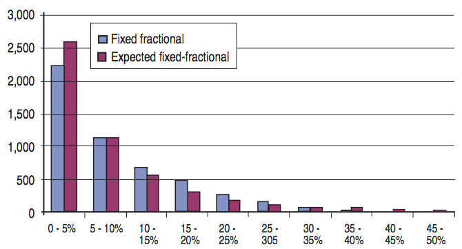
So in a nutshell – in reality trading systems will always lag behind their theoretical expectancy. Over time the difference actually adds to quite a bit of lost profits:

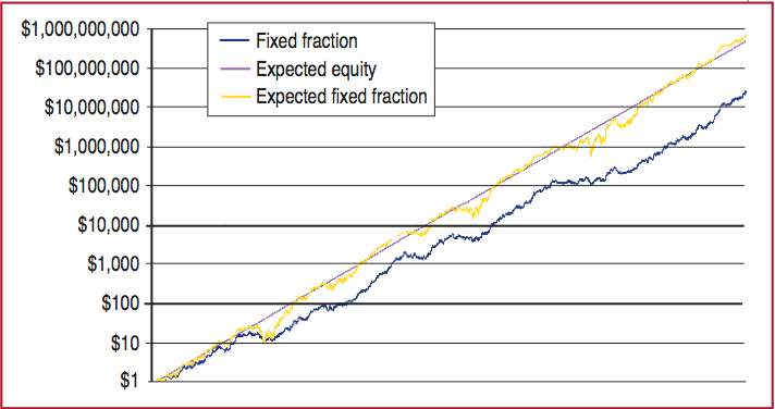
This graph is taken off the white paper and shows a Monte Carlo simulation of an hypothetical system over 5000 trades. Clearly this should not be taken as a realistic projection of a real life system and only serves to demonstrate the concept. The take away message is this: Over the life time of a system there is an exponential delta between its theoretical and geometric compounding results.

Clearly missing out on ill-gotten gain is not a situation we take lightly here at Evil Speculator. So I sat down and actually produced a handy spreadsheet which I invite you all to download and have a go with on your own. I’m only mildly versed in Excel and if you are able to offer an improvement then please share it with the rest of us. Now as you know I have quite a few systems in the running and what I wanted to find out if and how they would be affected. The results quite frankly were a bit surprising.

You may recall that I am currently live testing Scalpius which despite its name is more of an intra day swing trading system. It is based on some of my work on volatility cycles and thus far it’s looking extremely promising. After painstakingly running the stats on 10 forex and futures symbols over the past five years I arrived at the following stats:

• Win/Loss Percentage: 1:1.11 – which is 47 to 53.
• Average Win: 1.23R
• Average Loss: 0.76R
• Expectancy: 0.18R

The stats slightly vary between the various symbols but not excessively. There is a common theme which Scott often refers to as a ‘forest of good numbers’ – a term I really like as it describes the process of testing for possible system form fitting. I would characterize Scalpius as having a small but consistent edge. It won’t make you rich overnight but if you keep it in the running and if you are able to grab good fills then it’s a very promising system..

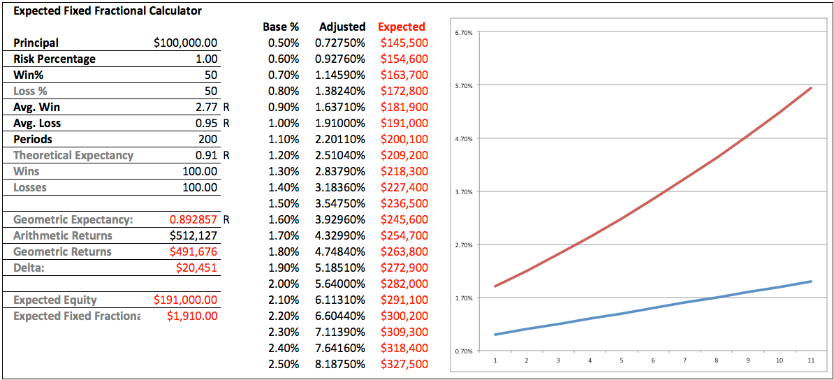
Now if you ran Scalpius via 0.5% fixed fractional position sizing (FFPS) then you would theoretically bank a $147k profit over 1,000 campaigns based on a theoretical expectancy of 0.1815R. Yes, that is just a theoretical model – we need to be clear on that. In any case, when comparing that with the geometric expectancy of 0.1765R we arrive at geometric returns of $144k, the delta in US$ being $3,031. Not exactly chump change but given the overall context it represents only 2% of the theoretical returns, thus I’d submit it to the BFD department and move on.

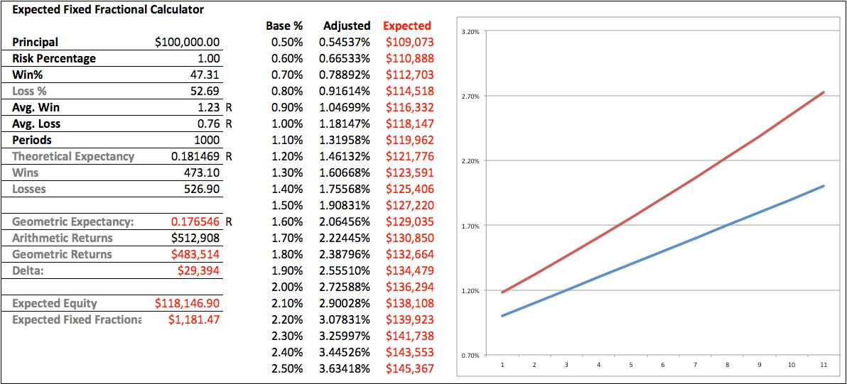
However look at what happens when we increase the base risk percentage from 0.5% to 1.0%. Suddenly the numbers jump quite a bit. Obviously larger position sizing increased the compounding effect significantly but the delta between the arithmetic and geometric returns now amounts to 5.7%.

And in order to compensate for the loss in profits our position sizing has increased accordingly. If you look at the table in the center of the graph then you will find that the difference in position sizing has to increase alongside the base percentage. Whereas compensating expectancy loss at 0.5% only requires a small increase to 0.545% at a base of 1.0% you are now required to trade at 1.18% position sizes relative to your actual equity, as that percentage represents 1% of your ‘expected equity’.

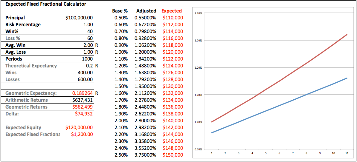
But there’s more to this story yet. If you read the white paper then you remember that Dr. Smart used the standard hypothetical 40/60 – 2:1 system for his Monte Carlo simulation. I have used those stats in the graph above but have taken the liberty to reduce the risk percentage to 1.0%. Quickly apparent is that this system has a better expectancy of 0.2R which in turn changes the dynamics of the delta between arithmetic and geometric returns. We’re are banking a bit more here obviously but if you look at the table in the center you’ll see that we are also using larger adjusted position sizing. Now instead of $100k we are calculating at an expected equity of $120k. That’s a 20% increase and those numbers grow even more quickly as we are increasing the base percentage.

If you were to use 2% position sizing instead as per the white paper then you would have to calculate your positions via an expected equity of $140k. Also the delta between arithmetic and geometric returns has jumped to a whopping 35.3%! So clearly time is not the only factor that affects compounding. The higher the SQL of your system the larger the loss in expectancy. Which to most of us would be counter intuitive, but the numbers do not lie. Systems with a higher win/loss rate require increased position sizing in order to keep up with their theoretical expectancy.

Take Away Points

Given the above dynamics there are several considerations for system developers. The first one is whether or not compensating for geometric returns via an increase in position sizing is worth the added risk. The white paper makes it clear that the increase in position sizing does also increase maximum drawdowns.

I have not run the numbers on that end myself but judging by the paper’s graph it seems that it is roughly in sync with the increase in risk percentage. So if you’re trading at an 1.2% adjusted position size instead of 1% then it’s realistic to expect at minimum 24% maximum drawdowns instead of 20% at fixed fractional position sizing.

And given that the dynamics between theoretical and geometric returns are highly system specific answering the question of whether it is worth it depends, as always, on your personal risk profile. The real question then changes from whether or not to use expected fixed fractional position sizing (EFFPS) to how much compensation you are willing to allow for. And if nothing else we also need to embrace the fact that theoretical compounding becomes less efficient with increasing SQN. Systems with smaller but consistent edges (as for instance Scalpius) actually benefit quite bit more in comparison with high expectancy but low opportunity systems.

Meaning, if you could choose between a holy grail system which trades 200 times per year and produces 100R and one that takes 1000 entries to produce the same 100R then most of us would probably instinctively choose the former over the latter. The graph above shows such a hypothetical system – I have fiddled with the stats to produce almost exactly the theoretical returns of what Scalpius is promising at 1% position sizes. The delta between the theoretical and geometric returns is smaller, but look at the position sizing required to keep up! At a base of 1% we would have to use 1.91% to account for a 3.9% difference. Hardly worth the additional risk I would say and I’m pretty sure most of you would agree.

Finally the more risk you are willing to take trading any system the higher will be the additional risk incurred in order to keep up with theoretical compounding. Increasingly larger position sizing means that draw downs will be deeper and generally your system will exhibit higher standard deviation. That is never a benefit to any system but especially systems that thrive via large outliers will be the most negatively affected. Drawing from some of the lessons we’ve learned about equity curve filters I believe that low dependency low standard deviation systems would benefit the most (e.g. Scalpius) and high dependency high standard deviation systems benefit the least from EFFPS. Reason being that a high number of consecutive losers will quickly do you in if you’re trading 3%+ position sizes.

The final take away is that we as traders need to be careful what we wish for. At some point in our career all of us have been on a hunt for that holy grail system which prints money fast with a small amount of trades. Given the inherent power of compounding it remains that elusive path to quick riches which many of us hope for but very few ever achieve (and the one’s who do aren’t talking).

Over the years I however have slowly shifted away from that and am now more focused on creating systems which produce a small but reliable edge over time. And apparently when it comes to compounding it is these types of systems which require the least amount of risk when it comes to compensating for exponential lag due to the delta between theoretical expectancy and geometric expectancy. On paper lofty outlier systems may seem what you want but given enough opportunity (i.e. number of trades) ‘more realistic systems’ with a consistent edge may actually rival hypothetical ones over time courtesy of compounding. Quite some food for thought.

Shameless Plug

It’s not too late – learn how to consistently bank coin without news, drama, and all the misinformation. If you are interested in becoming a subscriber then don’t waste time and sign up here. The Zero indicator service also offers access to all Gold posts, so you actually get double the bang for your buck.